Monday 20 February 2017

A script for turning Sheets data into Calendar entries (part 5)

Here is the final step in turning homework tweets into Calendar entries. Catch up here...
The gist of this step is that adding a new line to the top of a course's "hw to calendar" Sheet triggers a script that turns the info into a Calendar entry. (This is why the tweets are listed in order of date+time tweeted and not the due date.)

There is probably a way to do this from within the master "Tweets by @Ms_McPhee" Sheet, but when I was setting this up last summer, I couldn't find anything straightforward apart from this script I grabbed from a blog post (which I've lost the link to, so thank you anonymous blogger for your help). I know just enough about coding to add to someone else's code, so it may be clunky, but it works.

When I was testing this last summer, I had no difficulties. Naturally when school started and I was tweeting in earnest, a couple of strange little bugs appeared. Namely, each time the Sheet changed the script ran twice and I got two identical Calendar entries. Also, any time I tweeted anything, homework or not, or was retweeted, or was even mentioned in a tweet, it "changed" the Sheet (even if there was no actual change to the content), triggering the script. Twice. Which created more identical calendar entries. Sometimes I would have upward of 12 identical homework (or even worse, test!) entries on one day. Some of the students were a little startled, and I was spending far too much time in Calendar deleting superfluous entries.

To solve the second problem, I threw in a validation process. You'll need to add the following formula to cell M1:

=COUNTUNIQUE(C:C)

N1 also has a number in it, added by the script; you should leave it blank to begin with. The script now checks the number of essentially non-blank (or unique) rows and compares it to the number in N1. If N1 is less than the number of rows (meaning we've just added new homework information to the Sheet), it will run the calendar function and set the number in N1 to the number of rows. Otherwise, it's a fake "update" and the script can ignore it. It works well; now I can participate in Twitter chats without stressing out my students in the Calendar. The only thing I have watch is when I tweet out similar homework for different sections of a course to make them slightly different; usually all I need to do is change a punctuation mark.

I haven't worked out what's going on with the double posting, though. It now seems to be happening more or less randomly.

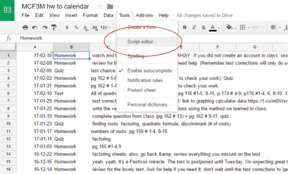
Here's how to  get the script running. From the Tools menu, select "Script editor."
screenshot of tools->script editor

A new window will open. Delete the older code, and copy the code below in its place . it's a wee bit long, because my rule is to never delete anything but instead comment it out in case I want to use it later. I grabbed most of this from the internet; the main thing I added is the row counter business.

I'll explain what a few of the lines do. In general, a // in front turns the rest of the line into a comment and a semi-colon finishes an instruction.
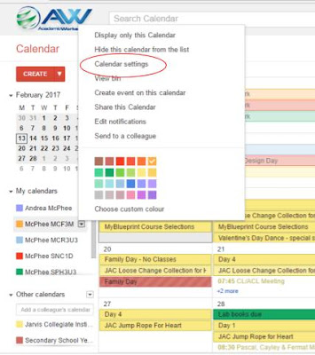
  • Row 4 tells the script which calendar to use. To get the calendar id, click on the triangle next to the desired calendar and choose Calendar settings.
screen shot of calendar settings

Scroll down to where it says Calendar Address. It's the code next to "Calendar ID," oddly enough. Copy that into the space between the quotes.


  • Rows 8-22 say which columns contain which pieces of information is in. It's a letter-to-number cipher, so A=1, B=2, etc.The start date is in column 1(A), the title in 2(B), the description in 3(C), the row counting cells are in 13 & 14 (M & N).

Rows 24-55 are the main script function, getLatestAndSubmitToCalendar, which is pretty much what it says on the tin.

  • Rows 26-32 get information about the sheet, including the number of  rows (which I don't think I need, but they were in the original script and so I left them. I'm not sure why). The original script took the information from the last row of the sheet, but importrange() turns that into a bottomless pit, which is why I reverse sort them.
  • Rows 34-47 get the actual date, title, description, and row-counting information from the Sheet.
  • Rows 50-55 run the createEvent script only if a new row has been added to the Sheet, and updates N1 to match the number of rows so a new calendar event won't be created if some other "change" is made to the Sheet.
Rows 57-70 are the createEvent function, which actually creates the Calendar entry. This is pretty straightforward. I set it up to create all day events because I think it makes the Calendar look less cluttered.


Before you can release it into the wild, you need to give your script permission to muck about with your Calendar. Save the script with a useful filename, then click Run -> getLatest...Calendar. During this run, a box will pop up asking to allow permission for the script to change your Calendar, etc. Let it. Then run it again to make sure it's working smoothly. I usually check it by manually changing N1 back to 0 (or one less than the number of unique rows), running the script again, checking that N1 has been changed, then checking the Calendar to see if the entry was created. You should get email notifications if the script fails to run.

The last step is to set the trigger. We want this script to run every time a new row is added (that is, when the Sheet is changed). Click on Resources -> Current project's triggers, or the stopwatch icon. If no triggers have been set, click on "No triggers set up. Click here to add one now.".  Make sure "getLatest...Calendar" is selected under Run. Under Event, change "Time-driven" to "From spreadsheet," then choose "On change." Save the script, test it out by tweeting something, and you're now automatically turning your tweets into calendar entries.


So there you have the somewhat involved process of turning tweets into Calendar entries. Please let me know if you have any questions or  suggestions -- especially about that nefarious double-trigger issue!

Friday 17 February 2017

Importing data to a new Sheet (part 4)

Update 17-03-17: Since originally writing these posts, I've learned more about what query() really does, so I'm updating some references.

Part 4 of an going series dealing with taking tweets about homework, sorting them, putting them on the course website, and creating Calendar entries. The story so far...
This (mercifully short) post will talk about how to link data in a parent Sheet to a completely separate Sheet. I need to have a separate Sheet for each course to run my calendar script, but there are any number of reasons you might want to link Sheets instead of just making a copy. If you want to embed only certain columns or tabs in the new Sites or in Classroom, it's easier if you import the data into a new Sheet first. The other reasons all pretty much have to do with the fact that if you make a change to the data in the parent Sheet, the new Sheet will update as well; a copy is not linked and won't update.  

It's really easy to do. Create a new sheet (I call mine "CourseCode hw to calendar") and copy the following code into cell A1:

=query(IMPORTRANGE("1hgVADAoR-TlKYPGawmMCmxaQKZ77lkKpbSdNozjzcCQ","Tweets for MCF3M!U:W"))

Importrange() will link to the data in a separate Sheet; it will update when you open the spreadsheet. (Query() lets the spreadsheet update without you having to open it, which is what automating is all about. sort/filter the data and is not strictly necessary here.) You will need to change both the red and the blue text for your Sheet.
  • The red text is the spreadsheet key of the main sheet, which you get from its url: https://docs.google.com/spreadsheets/d/1hgVADAoR-TlKYPGawmMCmxaQKZ77lkKpbSdNozjzcCQ/edit#gid=652985193
  • The blue text is the name of the tab you are getting the data from, followed by a ! and the columns you want. In this case, it brings in the columns with the sorted and reverse-dated tweets.
Note: When you're setting up the spreadsheet for the first time, you need to give access to IMPORTRANGE() first.*

screenshot of #REF! error: 'You need to connect these sheets.'

Give permission, and wait for your new sheet to populate...

screenshot of "adding permissions"

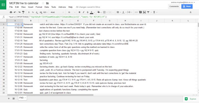
Once permission has been granted, you'll have a nice Sheet you can embed (or run a script on) with no worries. Any changes to the linked cells in the parent Sheet will automatically update in this one.

screenshot of populated imported data

The final installment of this series will talk about the script to create calendar entries from this data.

*At the beginning of the year, for each sheet I set up importing from the main one, I needed to copy the importrange part into another cell of the spreadsheet, click on the red error triangle, allow access, then delete that cell. When I was trying to grab screenshots for this post, new sheets already seemed to have access to the main one, which was a nice surprise. It looks like my setup time for new courses will be slightly reduced!

Monday 13 February 2017

Publishing a Sheet to the web (part 3)


Previously, on equals mc2...
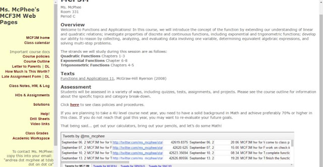
screenshot of website; click on my course pages above, pick a course, click on 'Class Notes' in the sidebar, and scroll down.

In this post I'll show you how to create the code to create a link to a webpage of (or embed) Sheets* data and talk about some things you have to watch out for. The 'Publish to the Web' feature is the other thing** that makes not just Sheets, but all of the GAFE tools supremely useful. I use it for lots of things, including self-grading quizzes and drill sheets, but I'll talk about it in the context of embedding my sorted homework tweets on the course webpage.

Update 17-03-17: You could probably do a lot of this with something like Awesome Tables, but if you're a noodler like me, you might do it this way.

Something to note: publishing to the web lets anyone who can visit your webpage (or who has the link) see your data; it makes a copy of the sheet and that's what is published. Any permissions you had on the original Sheet won't be copied over, and people might be able to see the underlying data for charts.

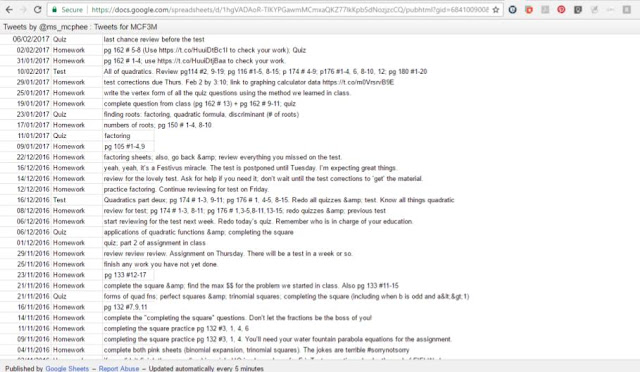
First, decide whether you want to create a web page, PDF, or a spreadsheet format, or if you want to embed the Sheet/tab*** in an existing webpage. Embedding a sheet looks like the screenshot above. Publishing it as a separate webpage looks like this:
single tab of sheet published to website

Here's how to do it. I'll talk about creating a link first, since embedding means a bit more work if you have columns to hide.

If you want to link to only part of a tab or more than one of the tabs (but fewer than all) in a sheet, you have to hide everything you don't want seen. Highlight any columns you want to hide (in the case of the homework tweets, that would be columns A-T), click on the triangle in the column header, and select "hide column."  If you want to share multiple (but not all) tabs, click on the triangle on the tabs you want hidden and select "hide sheet." Bear in mind that if you unhide anything, it will be visible on the web until you hide it again. I also take the time to get rid of the gridlines to keep it looking uncluttered.

Once you've taken care of that, you're ready to publish. Click on File->Publish to web.
screenshot of publish to web under file menu

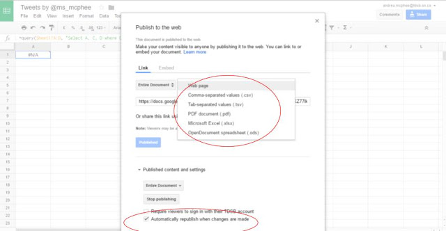
The default choice is to create a link to a web page, but you can also create a PDF.
screenshot of types of output

The "automatically republish when changes are made" should be checked -- unchecking it creates a static page that won't update.

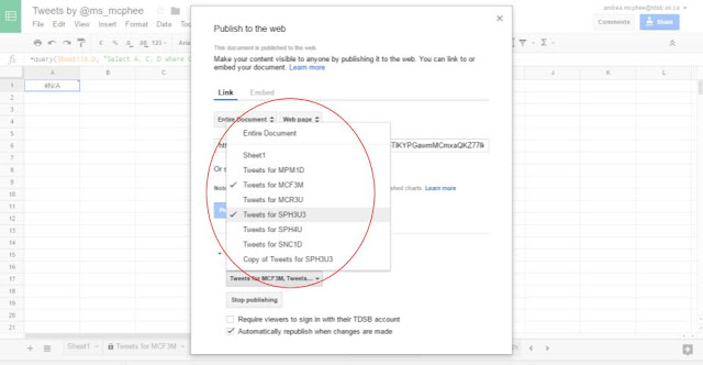
If you only want to publish one tab at a time, select it from the list. If you want to publish more than one tab in the same page, select "Entire document."

screenshot of selecting a few tabs to publish

I've been playing around with this a bit, and if you select several tabs from the lower menu, it will only publish one tab at a time. It looks like if you want to publish each tab separately, you have to close the 'publishing' pop-up and reopen it, choosing a separate tab to publish (getting an entirely new link). You would need to check off each tab you want to publish from the lower menu. However, I might be wrong and it might stop publishing the previous tabs. (I should say that I import my columns U-W into an entirely new Sheet for each course because of the calendar script, so I don't have to worry about hiding columns and I have only ever published one tab at a time from any given sheet.)

Here's what it looks like if you publish more than one tab at the same time using "Entire document." The user can click the links at the top to visit the different courses.
screenshot of sheet published to website (multiple tabs)
In the above example, I tried choosing to publish only the first four tabs, but it published the last one anyway. I hid Sheet1 and another tab, and as you can see they didn't get published. Hide what you don't want others to see, because the selection defaults to only one tab or the entire (viewable) document.

Any time you change the original Sheet, the webpage (or PDF, etc.) will also update. If at any time you want to stop publishing the Sheet, go to the publishing tab and click "Stop publishing" at the bottom. That way even if someone still has a link, they'll get a "We're sorry; that page is not published" error message.

Embedding a Sheet works the same way for the most part, except that you get html <iframe> code that you add to your site or blogpost. The main difference is, because you're embedding a copy of the Sheet, it will publish every column, including any you have hidden. To fix this, you need to either a) bring only the desired information into a new tab or Sheet and embed that (this is what I do) or b) manually add code to limit the range you embed. This post from hellotumo.com explains how to do that.

You will need to manually add width and height codes since the default is pretty small. I add width="90%" but keep the height the same since I only want the most recent homework tweets to be visible; users can scroll down to see older tweets. The code will look something like this:

<iframe src="https://docs.google.com/spreadsheets/d/1hgVADAoR-TlKYPGawmMCmxaQKZ77lkKpbSdNozjzcCQ/pubhtml?gid=769621547&amp;single=true&amp;widget=true&amp;headers=false" width=90%></iframe>

Below is what happens if you embed a sheet (with multiply tabs) and try to hide columns.
screen shot of embedding multiple tabs

I did hide columns A-T in the original sheet, but embed doesn't care. It does care that I hid a few tabs, which is nice of it.

In my next post, I`ll talk about how to import data from one Sheet to another. The final post will deal with the script to create a Calendar entry.

*If you are using Sites or Classroom, embedding the Sheet is easy; however I recommend importing the relevant information (such as the formula for column U) into a new Sheet since there doesn't seem to be a way to embed only one tab without hiding the rest and it won't let you hide the other columns. Here's hoping that the new Sites gives us an html code widget soon.

**The query() function being the best thing, of course. Oh, and that collaboration business.

***Again, by "tabs" I mean the different "sheets" within any one "Sheet," because that's just confusing.


Thursday 9 February 2017

Sorting course tweets in Sheets using query() (part 2)

Update 17-03-17: Since writing these posts, I've learned more about how query() actually works and the joys of arrayformula(), so I've updated some references below and modified the code at the bottom.

PS: TDSB teachers! Don't forget about Google Camp 4.0, March 4. Register on Key To Learn.

In this post, I'll discuss the nitty-gritty of how I take the tweets gathered by IFTTT into a Google Sheet and sort them out, ready to embed them by course on my website (see this post for an overview of the process).  I use them for homework tweets, but this information is useful for any data you've gathered into a spreadsheet (say, using Forms) and want to separate the information and embed the results somewhere. I can see it being used for sports teams, different subjects for one primary class, lesson plans, etc.

I've taken screenshots of my formulas and sheets and will go through in detail what each cell does. At the end of the post, I've written the formulas in a form that (hopefully) you can cut and paste into your own sheet, as well as links to a couple of my sample sheets so you can see what they look like. I'll talk about how to embed them and  the script to turn them into calendar entries in upcoming posts. This one will be long, image-heavy, and detailed. You have been warned.

First, a note about vocabulary. The tabs at the bottom are called 'sheets,' as in Excel, but since the whole thing is also called a sheet and that will get confusing, so I'm just going to call them tabs.

Once you've set up your IFTTT recipe to collect your tweets, open a new tab and rename it to your first course name. I use "Tweets for Coursecode," but the name isn't that important; you can do it by period or subject, or team, depending on how you want to separate your tweets. Recall that I structure my tweets thusly:

CourseCode hw for next day:: what needs to be done. for regular homework tweets and CourseCode quiz date_in_accepted_format:: what's on the test/quiz or review. for tests and quizzes. For example:

SPH3U3 hw for Fri:: prepping for presentation; continue reviewing for test.
MCR3U quiz 2017-02-07::simple vs compound interest

The first line of formulas goes from column A to U.  I'll break this into two parts: from A to L and from M to U.
screenshot of Sheets formulas; see bottom of post.

Here's what each cell does:
  • A1 uses query() to pull the date/time, content, and link of each tweet with the given course code (in this case, SPH3U3) into the tab. Column B in Sheet1 is the tweeter's name; since I'm only pulling tweets by me, I don't need it. I don't really need the links, either, but they help me differentiate between real and fake tweets (more on that in a bit). A holds the date and time.
  • B1 and C1 are empty, waiting for the content and link data from Sheet1.
    • A quick comment about query(): it's one of the coolest things about Sheets and what elevates it above stand-alone spreadsheets. It turns your Sheet into a real-time database, which means that everything I talk about below is automated without your having to open the spreadsheet. Set it and forget it. I'll do a future post about my love for query() and everything I use it for if you don't get a chance to catch my Sheets workshop at Google Camp 4.0. Update 17-03-17: Don't get me wrong, query() is still awesome, but it's Google itself that lets you set it and forget it. The awesomeness of query() comes from the way it lets you filter/sort and do math on data at the same time. Here, we're just using the filter & sort bits.
  • D1 is just a spacer.
  • Update 17-03-17: It's not in the screenshots, but I've added arrayformula() to each of cells E1 through Q1. What it does is let me do away with that copy-paste thing.
  • E1 turns the date and time into decimal values and adds them together. I use this to order the tweets in columns U-W so the most recent is on the top. This is only needed for the calendar script.
  • F1 uses the split() function to take cell A1 ("October 13, 2016 at 10:54") and separate it into date and time. F holds the date.
    • A few notes about the split() function: 
      • It's case-sensitive.
      • if you leave off the 'false', it will split the string at every separate instance of  each individual character of your splitter. In the above example, split(A1," at ") would result in "Oc", "ober", "13,", "2016", "10:54" because it will break the string at the first t, each space, and at " at "). Let's just say that can get super-fun when you're splitting using a word containing the letter e.
      • Notice that splitting the string leaves out whatever your splitter is.
      • You need to leave enough columns after the column with split() to contain all the separated parts, otherwise it won't work and you'll get a #REF! error ("Array result was not expanded because it would overwrite data in O3", say.)
      • The split() function can't handle blank cells, so until you have something for it to split, it will return a #VALUE! error. Don't worry about it.
  • G1 is blank to hold the time data from F1's split().
  • H1 separates the content of the tweet into two parts. I use "::" as a splitter so that I don't accidentally break URLs apart. H holds the course code and whether it's homework, quiz, or a test; if none of these (and there's no '::' in the tweet), it will hold the entire tweet.
  • I1 contains the meat of the tweet. This is the part that will go into the description of the calendar entry.
  • J1, K1, & L1 are insurance spacers in case I need the extra room for some weird separation thing that I wasn't expecting. I haven't so far, but it's nice to be sure.

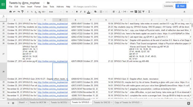
Here's what the first set of formulas look like with actual data: 
screenshot of the formulas in action; click on the link to the sheet at the bottom

Oh, so about those fake tweets? Row 28 in the screenshot above is an example; you can tell because there's no link in column C. Sometimes, especially when I'm extra busy and haven't scheduled my tweets, I forget to tweet out a quiz date or homework before the due date, but I still want it recorded. In that case, I just go into Sheet1, copy & paste the date/time format into the bottom row, make any changes I want, then type the 'tweet' content as usual. This is also how I test things out without going public on Twitter. And how it seems that I went back in time and tweeted about a quiz that had already happened.

The formulas for rows M through U look like this:
screenshot of Sheets formulas; see bottom of post.
  • M1 labels the tweets that are homework, quiz, or test (as opposed to general info or links). This becomes the title of the calendar entry. If it's none of these, it leaves the cell blank.
  • N1 is a spacer left over from when I was first playing around with how to do all this.
  • O1 is the cell that pulls the date of quizzes and tests out of the first part of the tweet. This is mostly for the calendar script: calendar entries for homework are created on the day it is tweeted, but tests/quizzes get entries on the day of the test/quiz. If this is a test/quiz tweet, it splits the tweet into two parts; otherwise it just uses the date of the tweet. I used "est" and "uiz" as splitters so I don't have to worry about whether or not to use capital T or Q. Incidentally, this only looks in H1 (before the '::', so I can talk about tests, quizzes, and estimations in the content of the tweet without worrying about it being split up).
  • P1 holds the date of the test or quiz, otherwise it's blank. It's important to tweet the date in Sheets-approved date format. Protip: 2016-12-14 is approved, 16-12-14 is not.
  • Q1 pulls all the dates into one column to make it easier to use query(). If P1 is blank, then O1 is the date of the tweet; otherwise, it takes the date from P1.
  • R1, S1, and T1 are just spacers.
  • U1 grabs the information that I'm going to embed in my website as well as turn into calendar entries. I only want the date (Q), title (M), and description (I), but obviously you could choose any columns in any order, For the calendar script, I need them listed by the order tweeted with the most recent on top so I use column E, but you could order it by Q if you wanted them by due date. U holds the date.
  • Leave columns V and W blank to hold the title and description.
Here's what they look like with data:


Looking at U26-28, you can see that the dates are out of order because I tweeted out the test date a week before.

In my next installment, I'll talk about how to take that information and publish it to the web, either by creating a link to a webpage or by embedding the Sheet. The last installment of this series will talk about the calendar script.

****

Here are the formulas for the first row in the course tabs in the original tweets sheet (Tweets by @Ms_McPhee). Copy cells B1:T1 down 100 or so rows (or however many you think you'll need; you can always copy more later). Do not copy cells A1 or U1. [Update 17-03-17: You don't need to copy these down because we are now using arrayformula()!] Change the information between the single quotes as needed. Until you have a tweet in the row, columns E, F, H, O, and Q will say "#VALUE!". This is because the split() function can't handle blank cells.
=query(Sheet1!A:D, "Select A, C, D where C contains 'SPH3U3'")=arrayformula(DATEVALUE(F1:f)+TIMEVALUE(G1:g))=arrayformula(split(A1:a,"at",false))=arrayformula(split(B1:b,"::",false))=arrayformula(if(isnumber(search(" Test ",H1:h)),"Test",if(isnumber(find(" hw ",H1:h)),"Homework",if(isnumber(search(" Quiz ",H1:h)),"Quiz","")))))=arrayformula(if(M1:m="Test", split(H1:h,"est ",false), if(M1:m="Quiz", split(H1:h,"uiz ",false),F1:f)))=arrayformula(if(isblank(P1:p),O1:o,P1:p)=query('Tweets for SPH3U3'!E:S, "Select Q, M, I where M='Homework' or M='Test' or M='Quiz' order by E desc")


Thursday 2 February 2017

Google Camp is coming...

Google Camp poster: I'm sharing Google Sheets: More than Just Number Crunching and Flipping Your Lessons: Tools and Tips

TDSB Google Camp 4.0 will be Saturday, March 4. At the risk of seeming like a Google Groupie, I love Google Camp; I've learned and been inspired by so much at every session I've attended -- not least during the demo slam at the end. I'm excited and more than a little trepidatious this year to be joining some amazing speakers. During the day, there will be a room with helpful helpers available if you've been running into difficulties with GAFE and need someone to walk you through the solution.

More info will be available soon at http://bit.ly/tdsbcamp, but TDSB teachers can register now through Key To Learn. This will sell out, so act now!