
I'm teaching MDM4U (Data Management), MAP4C (Grade 12 College), and MBF3C (Grade 11 College Math) this year (as well as three other courses, which perhaps explains the lack of posting). They all deal with, in one form or another, statistics. We're mostly using Fathom in MDM4U but for the other two courses I want to get them using Sheets, since they are more likely to see spreadsheets in the future than a proprietary statistical software.
One of the big downsides to stats in Sheets is the lack of box plots. Sadly, the apparently amazing Statistics add-on is not supported anymore, so we're stuck with what Sheets provides to us. Candlestick chart, which are intended for stock prices and graph low-open-close-high, could be used, but they are only vertical and don't include the median. You also need to put the data in horizontally, which I find counterintuitive.

They do give you a quick overview of the spread, if that is all you want.
There is a way to get something more box-and-whiskerish, and it's error bars to the rescue again. Here, we use a stacked bar chart:

It is by no means perfect, since the 1st quarter whisker is doubled (and as you can see sometimes goes past the box into the 4th quarter) and the 4th quarter whisker is reduced to a mere tick at the maximum value, but I think it does very nicely. I'm actually thinking it might be a better way to teach box plots, since there's a bit of prep to do beforehand that might make students pay attention to what it means. I haven't coded for outliers yet, and I think that will be less straightforward to include. Also, I don't think this will work at all if you have any negative values.
I am a little worried that some of my students will be confused by that extraneous right whisker in plot B, but we'll see.
To plot the data, you need to add an additional column per plot, like so:
The italicised numbers on the left are the what you would expect to plot on a box plot. The bolded values on the right N1:O6 are what you will actually plot. They are just differences between the points; J3 is just Q1 - Minimum for group A, and so on:

You can put in as many box plots as Sheets will allow, but you should keep the difference data, which is what you will plot, all together to make it easier on yourself.
Highlight the range of data Choose Insert -> Chart, then under Chart Type choose Stacked bar chart (Stacked column will give you a vertical box plot, if you like). Change the Stacking to "Standard" and select "Switch rows/columns". If you have labels for different plots in the first row, select "Use row 1 as labels".

Then click on CUSTOMIZE and choose Series. Here is where you will use the error bar and colour magic to make this thing look a bit more like a box plot.
The first box will be 0 to the minimum filled in. Choose "no colour" to make it disappear.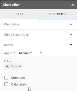

The second box, Q1, should be coloured a really pale colour. I use pale yellow. Select Error bars, make sure the Type is Percentage, and set the Value to 100. This will give you a whisker that goes all the way to the minimum value on the left (and Q1 + min on the right, unfortunately.)
You can leave the next two boxes (Median and Q3) as they are, or you can play around with colour choices. Keep them different colours so you can tell the difference between the 2nd and 3rd quarters, and I'd avoid choosing colours that are too dark because that extra whisker stands out too much.


Lastly, set the last box Maximum to the same pale colour you used for Q1. Select Error bar, keep the Type as Percentage, and set Value to 0. Sadly, if you choose 100 you'll get a right-hand error bar that goes beyond the maximum, which I think would be too confusing.
Note: this would be even better in Excel, which allows you to choose left or right error bars.
Next, you can turn the legend off, set the minimum value to be something a bit more in line with your data, and add some extra vertical gridlines if you like.
So there you go: quasi-box plots in Sheets. Let me know if you find this useful or have any suggestions for making it even better.

(This is what it looks like if you put 100% error bars in the Maximum box. Not worth the confusion, in my opinion.)
